Eventnet tutorial (case study: activity and attention in the collective production of migration-related Wikipedia articles)
Eventnet is now hosted in GitHub at https://github.com/juergenlerner/eventnet.
In this tutorial we illustrate how networks of relational events can be analyzed with eventnet and describe the most relevant options. For illustration we take a case study in which we analyze the collective production of Wikipedia articles by voluntary users. The description of eventnet provided by this tutorial, however, goes beyond the options that are necessary for this study. You might also have a look at the first steps tutorial for getting an overview about what eventnet does.
Study overview
In this study we analyze network effects that drive attention of contributing Wikipedia users to Wikipedia articles. In particular, we consider all articles in the English-language edition of Wikipedia that are in the category Category:Human migration or in a sub-category of it or in a sub-category of a sub-category. We consider this research setting as relevant since migration is a topic that is very high on the public agenda and Wikipedia is one of the most popular sources of information. However the main purpose of this web page is to illustrate the use of the eventnet software.The event network that we study is a two-mode network in which users interact with articles. We consider two types of events: edits to article pages and participation in discussion about article pages. The time of events is given by the second. We expect to find "network effects" in this kind of data in the sense that the rate of events from user U to article A likely depends on previous events on other user-article pairs. For instance, if user U already initiated many events, then this indicates that U is an active user and thus that the event rate on (U,A) is likely to be higher than average. Similarly if the article A already received many events, then it seems to be about a popular topic and the rate on (U,A) is likely to be higher than average. Moreover, we can expect local clustering in the sense that if two users often contributed to the same pages, then they seem to have common interests and are more likely to collaborate (potentially on different articles) in the future. This latter effect would be revealed by a tendency to close 4-cycles in the bipartite user-article network. Last but not least we are interested in dependencies between the two types of events, edit and talk. It could be that edit events trigger talk events, or the other way round, or both, or none. By this we can analyze whether editing tends to precede discussion, whether it is rather the other way round, or whether there are no interdependencies among the two types of events.
Readers interested in following the steps below can download these dyadic events at human_migration_events.zip (10.5 MB). You have to extract (unzip) this file on your computer to use it in eventnet. This event network consists of more than 950,000 relational events, connecting 87,000 registered users with 4,000 articles. The eventnet configuration with which the study can be reproduced can be downloaded at human_migration_configuration.xml (right-click and choose "save link as ...").
Starting eventnet and loading the configuration
(top)To follow the steps below download eventnet and start the program (open the graphical user interface), download the event file and possibly (unless you want to make all settings yourself) the configuration file.
To load that configuration into eventnet, use the file menu, choose merge into current configuration (if you want to preserve the current configuration, then choose open configuration) browse to the configuration file and open it. The minimal change in this configuration that you have to do yourself is to set the input directory (click on the browse button in the files-tab and locate the previously downloaded event file on your computer) and the output directory. It is advisable to choose an empty output directory or at least one in which there is no valuable data; better do not use the input directory as output directory. In general, eventnet might produce several output files whose names are assembled depending on the configuration settings. After these changes, you should already be able to execute the computation by clicking on the process button (left-hand side of the GUI). However, below we discuss the options (and their effect) in the six tabs of the eventnet GUI. See the first steps tutorial for an overview.
You can save a modified configuration via the file menu (or by typing Control-s). This allows you to continue after closing and restarting eventnet, to send the configuration to others for reproducibility, etc. Remember that the input data together with the configuration determines the output (up to potential random sampling).
File tab
(top)In the file tab you can set one or several input event files (or directories), CSV settings to parse these files, and an output directory. Different files can for instance contain events from different but comparable event networks. The results computed from different input files will also be written to different output files.
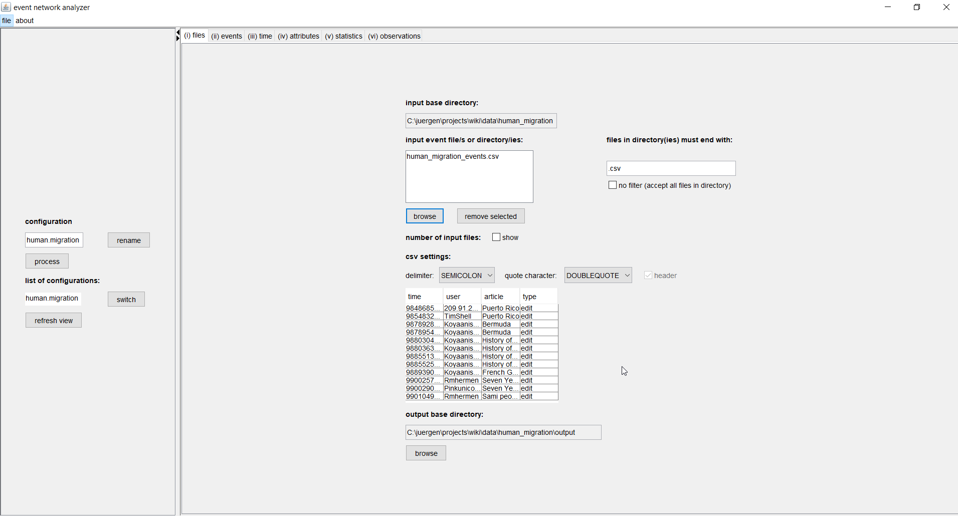
If you select several files then these must have a compatible structure. That is, components that are referenced in the next tab (events) must be present in all files and they must have the same column names. If you select directories, instead of files, then eventnet processes all files in the choosen directories. Additionally you can define that only files with a given ending (such as .csv) in these directories should be processed. If directories are selected then the output files will be written into respective subdirectories of the given output directory.
The delimiter in the CSV settings defines the character that separates one entry from the next. In our example, this is the semicolon. Quote characters are often used to enclose text that might contain (accidentally) the delimiter character. At the moment the input file(s) must have a header, that is, the column names must be explicitly given in the file. A preview table shows the first few lines of the input file. Wrong CSV settings often become apparent in this preview.
In the given example there are four columns named time, user, article, and type. One line in this file encodes that a given user contributed to a given article at the given point in time; the interaction type can be either edit or talk.
As indicated above, you should choose as output directory one that contains no valuable data since (assuming some bad luck with the file names) some of its content might be overwritten.
Event tab
(top)In the second tab (events) you can map the different components of an event to columns of the input file (or set them to implied) and define whether the event network is one-mode or multi-mode.
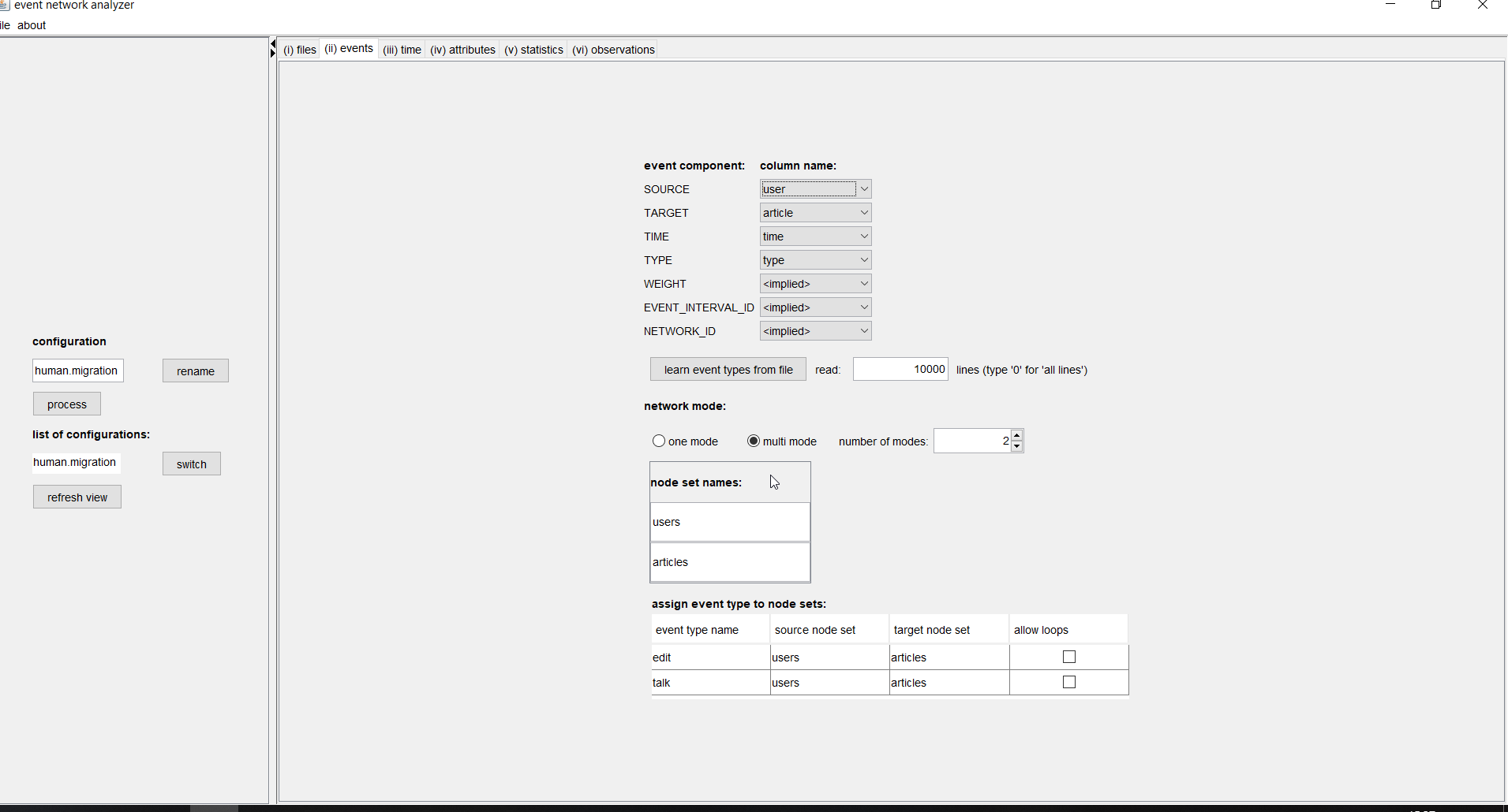
The seven components of an event are SOURCE, TARGET, TIME, TYPE, WEIGHT, EVENT_INTERVAL_ID, and NETWORK_ID. Only the source and the target must be given, the other components can be set to implied, with varying defaults for the different components. Even the source and/or the target could be empty for some events. For instance, events that happen on nodes (rather than on dyads), or events that set node attributes, could be given by events where the source or the target gives the respective node and where the other component is empty. The different components are explained in the following.
- (source) indicates who initiates the event. In our example the user is the source.
- (target) indicates who receives the event. In our example the article is the target.
- (time) gives the time of the event. Time can be given by integers, decimal numbers, or date-time strings such as 18.06.2018 or 2017-12-22T11:39:50Z. In the latter case, additional information about how to parse and interpret the data-time strings has to be given in the next tab (time). Events in the file must be sorted in time from the first event to the last event. (As an exception of that rule, see the network id component below.) Several events might happen at the same point in time; these are called "simultaneous events". If time is implied then events are implicitly numbered 1, 2, 3, ..., and these numbers are taken as the event time. In our example we have time given by integers representing milliseconds (the time precision is still seconds since the last three digits are always 000).
- (type) gives categorical (multinomial) information about what the source does to the target. If type is implied then it is implicitly equal to EVENT. In our example we have two types, edit and talk.
- (weight) is a decimal (or integer) number giving the strength, magnitude, etc of the event. If weight is implied then it is implicitly equal to one. In our example we do not have event weights. However, it would be thinkable that edit events have weight equal to the number of characters modified and talk events have weight equal to the number of characters of the user's contribution to the discussion page.
- (event interval id) is a string that marks sub-sequences of simultaneous events, where the simultaneity is not defined by the time variable but is externally given. For instance, if time is implied but we still have some information that certain events happen simultaneously. Subsequent events that have the identical value in the event interval id might be considered as simultaneous, dependent on settings in the next tab (time). In our example we do not have explicit event interval ids.
- (network id) is a string that marks sub-sequences that occur in the same event network. By default (that is, if the network id is implied) events in one file are considered as occurring in the same network. However it is possible to specify that events in the same file belong to different networks by providing a network id. In this case, all events in the same network have to appear consecutively in the file and events within a network have to be ordered in time. Events from different networks are considered to be independent of each other so that statistics explaining events in one network do not depend on any events from another network. Eventnet will use different output files for events from different networks, even if these are in the same input file. In our example we do not have explicit network ids so that all events in the single input file are considered to occur in the same network.
Apart from assigning (some of) the seven event components, you can also define whether the network is one-mode (that is, it has a single node set) or multi-mode (that is, it has two or more node sets). If the network is multi-mode then you can assign intuitive names to the different node sets. In our example, we have a two-mode network whose node sets are called "users" and "articles". If the network is multi-mode you have to map events types to pairs of node sets: one from which the sources of the events are taken and one containing the targets of events. Different event types (click on the learn event types from file button to enter the event types into eventnet) can occur between different sets of nodes. For instance it would be possible that events of some type occur from users to articles, events from a second type from articles to users, events from a third type from users to users, etc. Thus, multi-mode networks in eventnet are "mixed mode". In our example, however, we have that events of both types, edit and talk, have sources from the set of users and targets from the set of articles. Direct communication between users would be an example of events happening from users to users; however, we do not have direct communication between users in our example data. The check boxes allow loops are only relevant for types of events where sources and targets are taken from the same set. Obviously, if sources and targets are taken from different sets, then they cannot be equal and so there cannot be any loops.
The settings for multi-mode networks can also restrict the risk set, that is, the pairs of nodes on which an event of a certain type could happen. See the description on the observation tab for more information on this.
Time tab
(top)In the time tab you can specify the format of the time variable as given in the input file and you can define which events are considered as simultaneous.
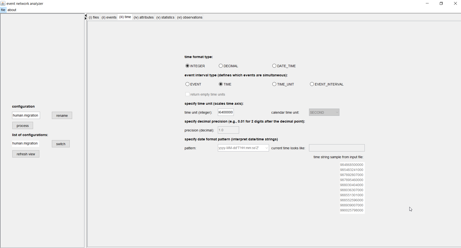
Time can be given by integers, decimal numbers, or date-time strings such as 18.06.2018 or 2017-12-22T11:39:50Z. In the latter case, additional information about how to parse and interpret the data-time strings has to be given by specifying a date format pattern, such as yyyy-MM-dd'T'HH:mm:ss'Z'. The date can be given in common or less common formats; see the java documentation for a detailed description (or ask us). To provide some guidance, eventnet shows the current date and time with the currently choosen date format and the first few time strings from the input file.
In our example, we have time given by integers, representing milliseconds since January 1st, 1970, at 0:00h.
The event interval type defines which events are simultaneous. The different options are
- (EVENT) each event happens alone
- (TIME) events with the identical time are simultaneous
- (TIME_UNIT) events in the same time unit (which might be an interval of any length; see below) are simultaneous
- (EVENT_INTERVAL) events that are assigned the same event interval id (see the discussion on the event tab) are simultaneous.
Assigning a time unit can make the time scale more intuitive. Actually millions or billions of milliseconds are not intuitive; days, for instance, are better. So, in our example, we set 86400000 as the time unit, which is the number of milliseconds of one day. Note that setting the time unit does not decrease the time precision. It just scales the time axis by defining what is one unit of time. If time is given by date-time strings then it is possible to set (multiples of) natural time spans (such as hour, day, week, month) as time units. If time is given by decimal numbers, a time precision has to be specified; for instance, setting the time precision to 0.01 results in considering two digits after the decimal point, setting it to 1E-10 would consider ten digits after the decimal point, etc.
If the event interval type is TIME_UNIT, then there is the possibility to also return empty time units. For instance, if the time unit is one day then there might be days on which no event happened. If the respective box has been checked, dummy events representing such empty time units will be generated. These empty time unit events might also generate observations (after all, events could have happened on these days). The dummy events have a flag so that latter components of the configuration (such as attributes or observations) can choose whether to respond to such dummy events or not.
Attribute tab
(top)Attributes record essential information about past events. Attributes are functions assigning numerical (decimal) values to dyads (that is, to pairs of nodes), to nodes, or to the whole network. The values of attributes, in general, change as time moves on. Attributes are used to define explanatory variables (statistics) that explain the rate of future events and/or to define the risk set (see the observation tab).
Eventnet provides common and less common types and variants of attributes. Among the most common are dyadic attributes that aggregate, separately for each pair of nodes (u,v), past events initiated by node u and directed to node v. For instance, such a dyadic attribute might simply count such events (potentially only events of a given type), it might aggregate the weight of such events, and it might have a decay that decreases the influence of past events as time moves on. Common node-level attributes might aggregate in-comming or out-going (or both) events of nodes and common network-level events might aggregate all events among any nodes, giving an indicator of the current activity level in the whole network. Attributes might also remember the time points of the last event (in the whole network, incident to a given node, or on a given dyad).
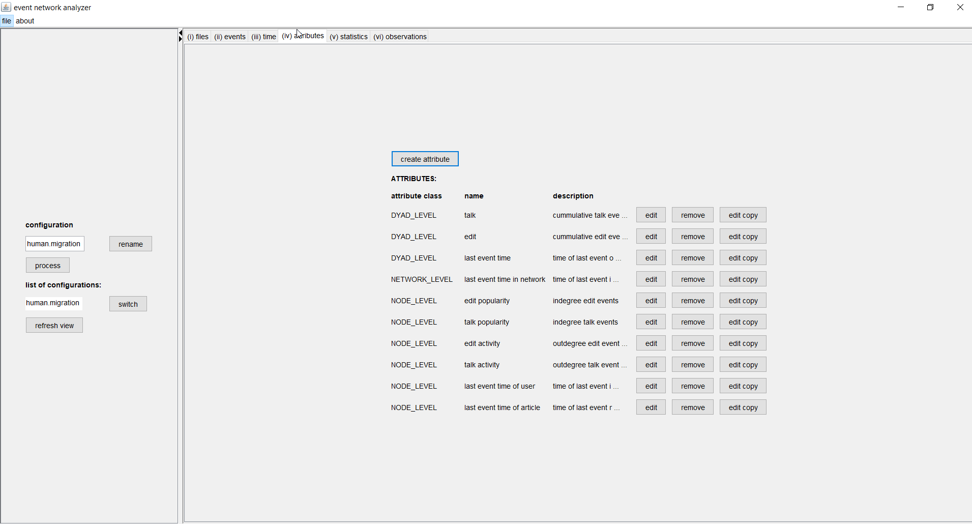
To create a new attribute click on the create button. Then you have to select the attribute class (dyad, node, or network) and then its type. A dialog opens in which the attribute can be defined. The list of attributes that have already been defined is shown in the attributes tab. Those attributes can also be modified (edit), removed, or a copy of them can be edited. The latter option is convenient if attributes share some common settings. In the following we describe the definition of some of the attributes used in our example.
The image below shows a dialog to define an attribute named edit which counts for each pair of nodes (u,a), where u is a Wikipedia user and a is a Wikipedia article, the number of past events of type edit from u to a, that is, the number of times user u edited article a before the current time. We have a similar attribute named talk which records the number of past talk events on user-article pairs.
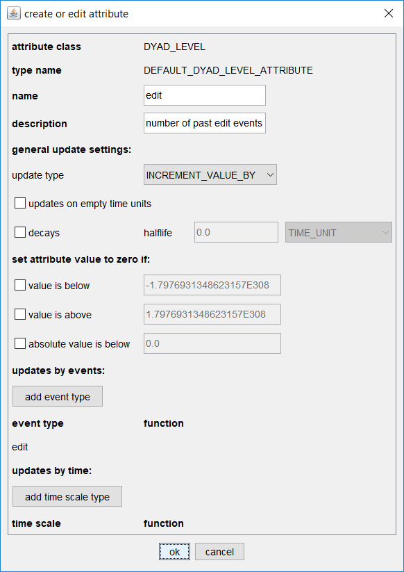
Only few of the possible options for defining attributes are used in this concrete example. For instance, attributes might have a decay which means that, if no update happens in between, their value gets halved whenever the time advances by a given halflife period. Attributes with a decay give more weight to recent past events. Attributes can also define that they are rounded down to zero if their value drops below a given threshold (which might happen due to decay).
The last two sections updates by events and updates by time can define types of events whose weights are used to update the current attribute values, or time variables that are used to update current values. As an example for the former option we add the weights of events of type edit to the current attribute value (these weights are actually equal to one in the given example in which event weights are implied). An an example of the latter option the attribute last event time records the time of the last event on a given dyad (readers are invited to look at the settings by clicking the edit button close to that attribute in the attribute tab). Common functions (or lists of functions) can be applied to transform weights or time variables before updating values.
Node-level attributes can aggregate in-comming or out-going events (or both) incident to nodes. In our example we have, separately for the two event types edit and talk, attributes for the activity (out-degree) of users and the popularity (in-degree) of articles.
Statistic tab
(top)Statistics are the variables that explain future event as a function of past events, that is, as a function of attributes defined in the attribute tab.
The predicted rate of events on a dyad (u,v) can depend on
- past events on (u,v), (v,u), or both (DYAD_STATISTIC)
- past events incident to u, v, or both (DEGREE_STATISTIC)
- common neighbors of u and v (TRIANGLE_STATISTIC)
- 3-paths connecting u and v (FOUR_CYCLE_STATISTIC)
- attributes of u or v (NODE_STATISTIC)
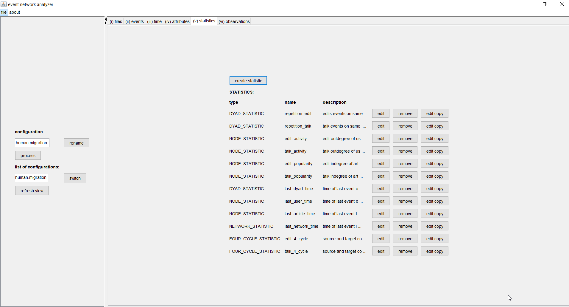
In our example we define as explanatory variables (statistics) dyad statistics, modeling the tendency to repeatedly contribute to the same article; degree statistics (actually operationalized as node statistics), modeling activity and popularity effects; and four cycle statistics, modeling local clustering of users and articles. We do not consider triangle statistics since we analyze a bipartite network. These statistics are defined separatly based on past edit events and past talk events.
Observation tab
(top)Observation generators (or short, observations) define the risk set, that is, the events that could have happened. Observations also provide efficient means to sample from the risk set (case-control sampling) which is appropriate if the number of non-events is much larger than the number of events.
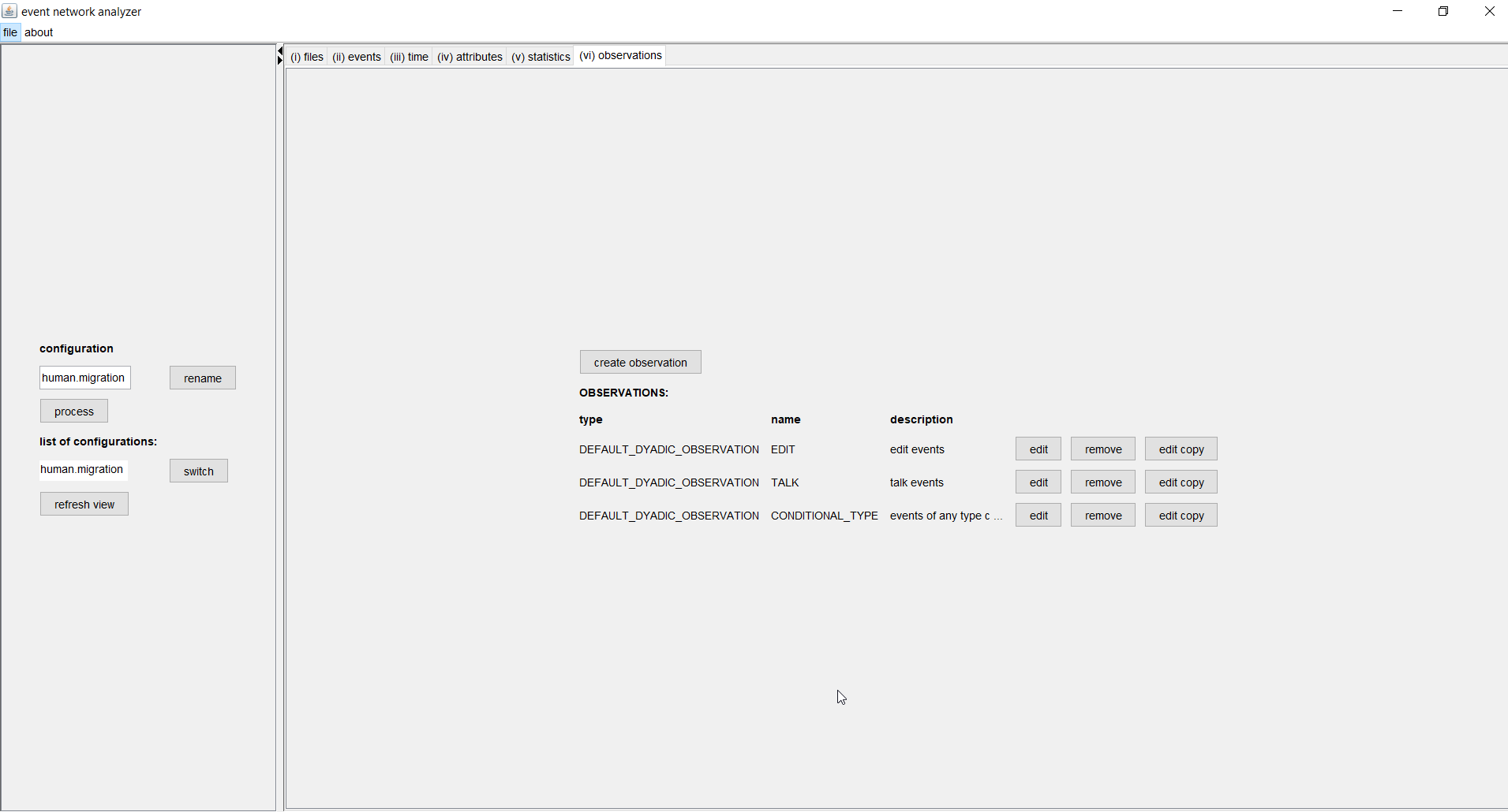
Eventnet can model observations on dyads or on nodes, can restrict observations to particular event types, require sources or targets to be from given sets (for multi-mode networks) or to be non-zero on given attributes (the latter option can model dynamic risk sets that might change as a function of events). It further allows to condition on observed sources, or targets, or both. In our example we have three observation generators: two modeling the rate of events of type edit or talk, respectively, and one modeling the conditional type of events, that is, the preference for edit over talk (or the other way round) given that users interact with articles. Possible settings can be seen in the dialog below.
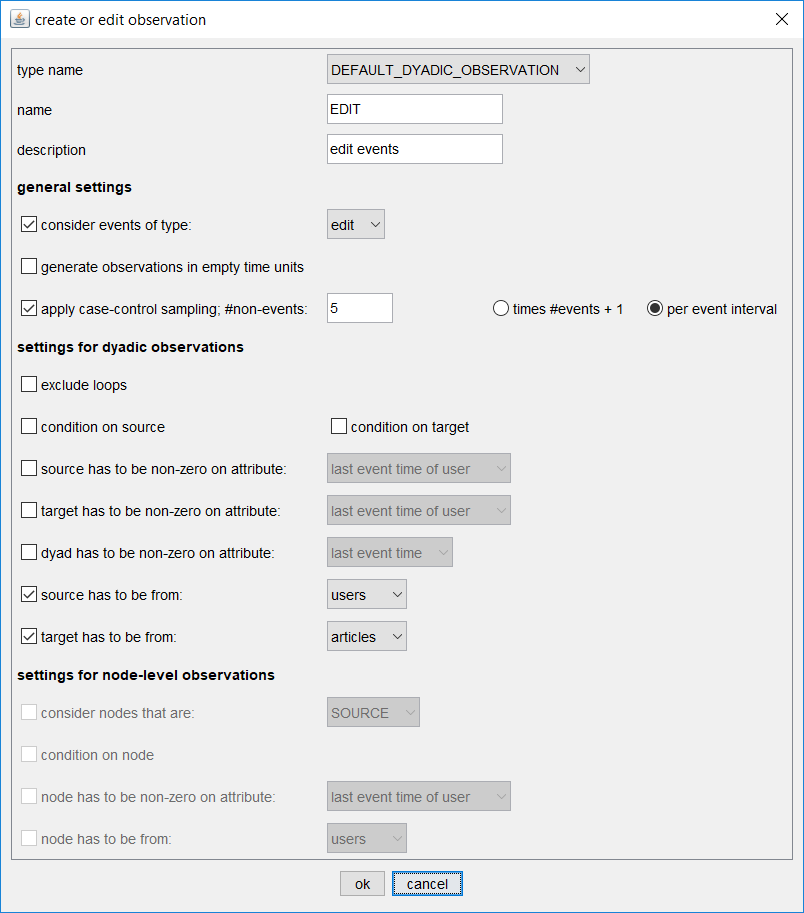
In the example above we define an observation generator named EDIT that considers all events of type edit. The risk set (that is the set of dyads on which an edit event could have happened at a given point in time are all pairs of nodes (u,a) where u is from the set of users and a is from the set of articles. This risk set is huge in our concrete example. The 87,000 registered users interacting with 4,000 articles yield 87,000 x 4,000, that is more than 300 million, dyads in the risk set. Around the end of the observation period we could, at any point in time, observe events on any of these 300 million dyads - but typically we observe an event on only one of these dyads. Case-control sampling has been proposed to deal with such an abundance of non-events. It samples all the events but only a given number of non-events. In our example we sample 5 non-events in each point in time in which an event has been observed (that is about 950,000 times). The reliability of this sampling procedure can be tested by sampling repeatedly and comparing differences between results (see below). Besides case-control sampling, eventnet also offers the possibility to sample from the observed events, that is, from the sequence of input events. This second sampling strategy becomes relevant when even larger networks should be analyzed. It is not necessary for the current study.
How the reliability of estimates under sampling (case-control sampling or sampling from the observed events) can be assessed is explained in more detail in the tutorial on analyzing large event networks.
The observation generator CONDITIONAL_TYPE conditions on the source and the target of observed events. The only "free" variable in this observation generator is the type of events. Thus we can model a user's perference for engaging in edit rather than in talk events (or the other way round), given that the user does contribute to a certain article at a given point in time. No case-control sampling is needed for this observation, since here we consider only observed events (there are no non-events to sample from).
A completed configuration can be executed either by clicking on the process button in the left-hand side of the eventnet GUI or - without opening the GUI - via java -jar eventnet-x.y.jar configuration_filename.xml (or, by java -jar -Xmx4g eventnet-x.y.jar configuration_filename.xml to increase the memory size to 4GB, etc). Results from different observations are written to different output files.
Analyzing the output files with R
(top)The following R code provides examples to analyze the three different output files (generated by the three observations). To execute this code you have to install the R software for statistical computing. It is convenient to use an R programing environment, such as R-Studio.
First load the R package 'survival'. Of course it is also possible to analyze the output with other software (than R) or with other packages for time-to-event data, or otherwise.
## install the R package 'survival' if necessary
necessary.packages <- c("survival")
missing.packages <- necessary.packages[!(necessary.packages %in% installed.packages()[,"Package"])]
if(length(missing.packages) > 0) {
  install.packages(missing.packages)
}
# attach the library
library(survival)
# increase the memory size, if you want
memory.limit(size=16000)
Set the directory name of the working to the directory that you have specified for output.
# set the working directory
# it is very likely that you have to adapt the following line
setwd("c:/juergen/projects/wiki/data/human_migration/output/")
Modeling the rate of edit events
A first relational event model is specified for explaining the rate of edit events on dyads.
## analyze EDIT events
# load the file containing observations and explanatory variables
edit.events <- read.csv2("human_migration_events_EDIT.csv", dec = '.')
# have a look at its content
summary(edit.events)
It can be helpful to standardize explanatory variables (that is, transform them linearly to zero mean and standard deviation equal to one) as this makes the sizes of estimated parameters more comparable.
standardize <- function(x){
  x <- (x-mean(x))/sd(x)
  return(x)
}

var.names <- names(edit.events)

for(i in 10:length(var.names)){
  edit.events[,i] <- standardize(edit.events[,i])
}
summary(edit.events)
These observations are analyzed with the Cox proportional hazard model. This model does not explain the time to the next event. Rather it explains that the event rate on some dyads is higher or lower than on other dyads. This model is appropriate for this situation since it filters out variation in the general activity in the given part of Wikipedia. An alternative would be the function clogit in the survival package.
## specify and estimate a Cox proportional hazard model
edit.surv <- Surv(time = edit.events$TIME, event = edit.events$IS_OBSERVED)
edit.model <- coxph(edit.surv ~ repetition_edit
                  + repetition_talk
                  + edit_popularity
                  * edit_activity
                  + talk_popularity
                  * talk_activity
                  + edit_4_cycle + talk_4_cycle
		  + strata(TIME)
                  , data = edit.events)
# see the results
summary(edit.model)
The important part of the estimated model is shown in the following.
  n= 4893882, number of events= 816653
                                    coef  exp(coef)   se(coef)      z Pr(>|z|)
repetition_edit                 5.017873 151.089623   0.018068 277.72  < 2e-16 ***
repetition_talk                 1.095822   2.991639   0.019522  56.13  < 2e-16 ***
edit_popularity                 0.924448   2.520478   0.005183 178.35  < 2e-16 ***
edit_activity                   0.966506   2.628745   0.004350 222.17  < 2e-16 ***
talk_popularity                 0.026544   1.026900   0.004439   5.98 2.23e-09 ***
talk_activity                  -0.237837   0.788331   0.003664 -64.91  < 2e-16 ***
edit_4_cycle                    0.034228   1.034821   0.004457   7.68 1.59e-14 ***
talk_4_cycle                    0.342908   1.409039   0.004554  75.30  < 2e-16 ***
edit_popularity:edit_activity  -0.257772   0.772771   0.002642 -97.56  < 2e-16 ***
talk_popularity:talk_activity  -0.088267   0.915516   0.003143 -28.09  < 2e-16 ***
---
Signif. codes:  0 '***' 0.001 '**' 0.01 '*' 0.05 '.' 0.1 ' ' 1
We see that all parameters are significantly different from zero. Some of the effects are as expected. For instance, we find a positive parameter associated with repetition_edit. This means that users tend to edit articles that they have edited before. We also find that both popularity effects are positive. This means that the more attention (expressed by edit or talk events) an article received in the past, the more edit events it is likely to receive in the future from potentially different users. Similarly we find a positive activity effect for users' engagement in editing.
Perhaps more unexpected is the finding that the statistic talk_activity has a negative parameter. This means that users who engage more in discussion (on any article) are less likely to edit - all other things being equal. Below we will see that conversely participation in editing tends to decrease engagement in discussion.
Importantly, we find negative interaction between article popularity and user activity. Thus, the more active users are drawn to start working on the less popular articles (that are otherwise in danger of being neglected, as revealed by the positive popularity effect).
Modeling the rate of talk events
Specifying and estimating a relational event model for talk events is very similar. For completeness we give the R code below.
## analyze TALK events
# load the file containing observations and explanatory variables
talk.events <- read.csv2("human_migration_events_TALK.csv", dec = '.')
summary(talk.events)

## standardize variables
var.names <- names(talk.events)
for(i in 10:length(var.names)){
  talk.events[,i] <- standardize(talk.events[,i])
}
summary(talk.events)

## specify and estimate Cox proportional hazard model
talk.surv <- Surv(time = talk.events$TIME, event = talk.events$IS_OBSERVED)
talk.model <- coxph(talk.surv ~ repetition_edit
                    + repetition_talk
                    + edit_popularity
                    * edit_activity
                    + talk_popularity
                    * talk_activity
                    + edit_4_cycle + talk_4_cycle
		    + strata(TIME)
                    , data = talk.events)
# see the results
summary(talk.model)
The findings from this model are shown are the following.
  n= 828145, number of events= 138080
                                   coef exp(coef)  se(coef)       z Pr(>|z|)
repetition_edit                 6.07522 434.94632   0.07536  80.616   <2e-16 ***
repetition_talk                 5.80326 331.37937   0.11977  48.452   <2e-16 ***
edit_popularity                 0.58953   1.80315   0.02168  27.186   <2e-16 ***
edit_activity                  -0.20523   0.81446   0.01698 -12.088   <2e-16 ***
talk_popularity                 0.46524   1.59239   0.02096  22.201   <2e-16 ***
talk_activity                   1.32778   3.77266   0.01873  70.888   <2e-16 ***
edit_4_cycle                   -0.36954   0.69105   0.01778 -20.779   <2e-16 ***
talk_4_cycle                    1.11960   3.06362   0.02395  46.747   <2e-16 ***
edit_popularity:edit_activity  -0.02620   0.97414   0.01174  -2.231   0.0257 *
talk_popularity:talk_activity  -0.65526   0.51931   0.01783 -36.753   <2e-16 ***
---
Signif. codes:  0 '***' 0.001 '**' 0.01 '*' 0.05 '.' 0.1 ' ' 1
As indicated above edit_activity has a negative parameter in the talk model. Thus, users who are more engaged in editing (on any article) are less likely to participate in discussion - all other things being equal. Thus, we find that users play different roles, some being more involved in editing articles and others contributing more to discussion. This is also revealed in the next model where we model the conditional type (edit vs. talk) of events.
Modeling the conditional type of events
A totally different kind of model is that for the conditional type of events. Here we model the conditional probability that a user u edits an article a, given that user u does contribute to article a in some way. The two possibilities to contribute (in our data) are edit or talk so that we model a conditional preference for edit over talk. Here we do not model whether u contributes to article a in any way. The data is loaded and preprocessed by the following commands.
## analyze the conditional event type
# have a look at its content
cond.type.events <- read.csv2("human_migration_events_CONDITIONAL_TYPE.csv", dec = '.')

# we want to analyze the preference of engaging in edit events over talk events
# create a binary variable 'is_edit'
cond.type.events$is_edit <- 0
cond.type.events[cond.type.events$TYPE == "edit",]$is_edit <- 1
Since in our data users can only choose among two alternatives we can use a binomial model. (More alternatives could be specified in a multinomial model.)
# specify and estimate a logistic regression model for the probability whether given events are edit events
cond.type.model <- glm(is_edit ~ repetition_edit
                    + repetition_talk
                    + edit_popularity + talk_popularity
                    + edit_activity + talk_activity
                    + edit_4_cycle + talk_4_cycle
                    , family = "binomial"
                    , data = cond.type.events)
# see the results
summary(cond.type.model)
The findings from this model are shown are the following.
                 Estimate Std. Error z value Pr(>|z|)
(Intercept)      1.164549   0.015295   76.14   <2e-16 ***
repetition_edit  0.250810   0.004552   55.10   <2e-16 ***
repetition_talk -0.455119   0.005563  -81.81   <2e-16 ***
edit_popularity  0.286872   0.004878   58.81   <2e-16 ***
talk_popularity -0.313301   0.004496  -69.68   <2e-16 ***
edit_activity    0.590215   0.004358  135.43   <2e-16 ***
talk_activity   -0.815573   0.004223 -193.14   <2e-16 ***
edit_4_cycle    -0.018701   0.001580  -11.84   <2e-16 ***
talk_4_cycle     0.046438   0.001542   30.12   <2e-16 ***
---
Signif. codes:  0 '***' 0.001 '**' 0.01 '*' 0.05 '.' 0.1 ' ' 1
What we find is first a positive intercept, resulting from the fact that we have more edit events than talk events. The parameters for the repetition, popularity, and activity effects are as it could have been expected. Past editing increases the relative probability of future editing (and therefore decreases the relative probability of future talk), while past engagement in discussion decreases the relative proability of future editing (and therefore increases the relative probability of future talk). The findings for the four-cycle effects go slightly in the other direction.
If you are interested in analyzing larger event networks, using different sampling strategies and assessing the reliability of estimates under sampling, see the tutorial on analyzing large event networks.